Predicting growth in children - part 1/2
What would happen if a doctor could know beforehand if a child is going to have health issues?
Let’s say a mother arrives with her baby at the doctor’s office to have a routine check-up. The doctor does his job and everything seems fine. He enters all the baby’s new info on the computer but it informs that the baby is probably going to be at risk… in about four months from now.
Today, this is still science fiction, but we are not THAT far from it. Today I’ll write about a competition I took part of, which addressed a similar problem: given some measurements like the weight or height of a baby, will those values be dangerously low in the future?
The problem to solve
In the context of the ECI week (School of Informatics Sciences for its initials in Spanish), a competition was launched in Kaggle which theme was children health analysis. The problem consisted of a dataset contaning routine check-ups for different babies in different regions of Argentina. Our job was to predict if the z-scores for height, weight and body mass (HAZ, WAZ, BMIZ from now on) will be below a given threshold in the next check-up.
The competition was open to everyone, it was an interesting problem and a good classifier will have a positive impact in national medicine.
Also, it has been a long time since I didn’t compete, so it was the perfect excuse for me to do so. sentiment_very_satisfied
Let’s look at the data
The dataset for this competition is pretty straightforward and small enough for running nice experiments. The train set has 43933 rows and the test set 6275 rows. Both sets have 23 columns (features).
Here are the first rows of the original train data:
-
[[{col.field}]]
| [[{user[col.field]}]] |
Here we have the description for each feature:
| Name | Description |
|---|---|
| BMIZ (float) | Body-mass-index-for-age-Z-scores (BMI standardized reference by age and gender) |
| HAZ (float) | Height-for-age Z-scores (standard reference of height by age and gender) |
| WAZ (float) | Weight-for-age Z-scores (standardized reference of weight by age and gender) |
| … | … |
| Name | Description |
|---|---|
| BMIZ (float) | Body-mass-index-for-age-Z-scores (BMI standardized reference by age and gender) |
| HAZ (float) | Height-for-age Z-scores (standard reference of height by age and gender) |
| WAZ (float) | Weight-for-age Z-scores (standardized reference of weight by age and gender) |
| Individuo (int) | Identifier assigned to each individual |
| Bmi (float) | Bmi = weight / (height ^ 2) |
| Departmento_indec_id (int) | Department code of the hospital. It matches the code obtained from INDEC |
| Departmento_lat (float) | Average latitude of the hospitals of said department |
| Departmento_long (float) | Average of the length of the hospitals of said department |
| Fecha_control (string) | Date the individual was checked-up |
| Fecha_nacimiento (string) | Date the individual was born |
| Fecha_proximo_control (string) | Date the individual will be checked-up next time |
| Genero | Gender of the individual (M = male, F = female) |
| Nombre_provincia (string) | Name of the province where the individual was attended |
| Nombre_region (string) | Name of the region where the individual was attended |
| Perimetro_encefalico (float) | Measurement of encephalic perimeter obtained in the attention (cm) |
| Peso (float) | Measurement of weight obtained in the attention (kg) |
| Talla (float) | Length measurement obtained at attention (cm) |
| Provincia_indec_id (int) | Province code (S = yes belongs, N = does not belong). |
| Zona_rural (string) | Code that indicates if the hospital is in a rural area |
| Var_BMIZ | Variation that BMIZ will have in the following attention regarding the current value |
| Var_HAZ | Variation that will have HAZ in the following attention regarding the current value |
| Var_WAZ | Variation that will have WAZ in the following attention regarding the current value |
Now let’s see what we have to predict. Our target variable is made of three conditions:
| Decae (Target variable) |
It takes the value "True" if at least one of the following conditions occurs:
{
HAZ >= -1 and next_HAZ < -1
WAZ >= -1 and next_WAZ < -1
BMIZ >= -1 and next_BMIZ < -1
|
This is, if the current value for the z-score is greater than -1 and in the next check-up it is less than -1 we can say that the value dropped below an acceptable range, and the baby is possibly at risk (and our target variable is true). Note that if the previous value was below -1, the next value doesn’t matter because our condition will always be false.
A couple of examples:
| HAZ check-up Jun '16 | HAZ check-up Nov '16 | decae |
| 0.12 | -1.02 | true True, HAZ was >= -1 and now is < -1 |
| -0.5 | -0.99 | false False, HAZ is always >= -1 |
| -1.5 | -1.8 | false Both checkups are below -1, the condition needs the first one to be >= -1 |
HAZ over two different check-ups
| HAZ Jun '16 | BMIZ Jun '16 | HAZ Nov '16 | BMIZ Nov '16 | decae |
|---|---|---|---|---|
| 0.1 | 1.0 | -1.5 | 1.0 | true HAZ dropped below -1 |
| 0.1 | -1.1 | -1.5 | -1.1 | true BMIZ is below -1 but this was true in the previous check-up. HAZ dropped below -1 and this is why we have a true. |
HAZ and BMIZ over two different check-ups
The row highlighted is false regardless of being below -1.0 because HAZ also was below -1.0 on the previous check-up . Here we have a dependency, the target variable depends on the value of the previous seen check-up , and it has to be >= -1 for the target to be true. This is a hard threshold/limit and we will explore what happens on some of the models we train with if we just ignore it, later in this post.
One last thing to mention is that the scoring metric that we will use is ROC AUC (interactive)
First things first
Let’s say Alice and Bob download the train set and start working. Bob’s idea is to have a good model, clean, with nice features and good hyperparameters before submitting a solution. Alice on the other hand thinks it’s better to be able to submit quickly and then improve the solution.
Bob works for a week before submitting, guiding his work on the results of his own validation set. However, the day he submits his solution, something went wrong and the score is lower than he expected. It could be a bug on his code, or maybe he overfitted at some point and now possibly has to go back to a complex to debug program.
Alice does just the minimal work to have a solution ready as fast as possible. She did a basic clean up of the dataset, ran any model with default parameters and generated the solution. She submitted and got a not-so-good score, but now she has a baseline on which to improve. She knows her pipeline works from end to end, she just has to improve the solution.
I’m not saying that anyone that does what Bob did will make a mistake before having a solution, but I think it’s better to have a working solution and then improve it. This is true for both competitions and the industry.
So I did exactly that, I cleaned up the dataset (basic imputation and labeling), ran a Gradient Boosting model with default parameters and submitted my solution. My baseline score was 0.77043 and it was enough to be on the top ten at that specific time!
Exploring the data
Before going any further a good idea is to actually see the data and think how it can help us solve the problem. If we were a doctor, how can we intuitively know if there’s something wrong with a baby? Probably measuring his weight, height, and other things could help. We can also see his socioeconomic environment, does he live in a zone with higher probability of leading to health problems? Ideally, we could also see his mother’s situation, is she healthy? Does she take good care of her baby?
We don’t have that last bit of information, but we have something about the first two parts. We have the weights, heights and z-scores and some geographic data that we can extrapolate with external socioeconomic data.
Let’s start with the z-scores. Here you can see some examples, and how they relate to the target variable:
    <a class='fancybox-thumb ' id="HAZ" title="HAZ"
       data-thumb="/assets/eci/haz.png" href="/assets/eci/haz.png" rel="density">
        <img alt="HAZ" src="/assets/eci/haz.png">
        <span class="fancy-caption">HAZ</span>
    </a>


    <a class='fancybox-thumb ' id="WAZ" title="WAZ"
       data-thumb="/assets/eci/waz.png" href="/assets/eci/waz.png" rel="density">
        <img alt="WAZ" src="/assets/eci/waz.png">
        <span class="fancy-caption">WAZ</span>
    </a>


    <a class='fancybox-thumb ' id="BMIZ" title="BMIZ"
       data-thumb="/assets/eci/bmiz.png" href="/assets/eci/bmiz.png" rel="density">
        <img alt="BMIZ" src="/assets/eci/bmiz.png">
        <span class="fancy-caption">BMIZ</span>
    </a>
We see that, between certain points, we have more density of cases with the target variable on true. This could be useful later if we can encode this information into our model.
Here is a simple exploration of the features:
| Feature | top | freq | mean | std | min | 25% | 50% | 75% | max |
|---|---|---|---|---|---|---|---|---|---|
| BMIZ | — | — | 0.491 | 1.277 | -4.935 | -0.307 | 0.524 | 1.323 | 4.997 |
| HAZ | — | — | -0.662 | 1.323 | -5.996 | -1.450 | -0.612 | 0.173 | 5.997 |
| WAZ | — | — | -0.021 | 1.177 | -5.853 | -0.717 | 0.030 | 0.742 | 4.872 |
| individuo | — | 4 | — | — | — | — | — | — | — |
| bmi | — | — | 17.333 | 2.210 | 8.3298 | 15.938 | 17.301 | 26.874 | |
| departamento_lat | — | — | -29.672 | 3.278 | -38.976 | -32.527 | -27.551 | -26.838 | -25.402 |
| departamento_long | — | — | -62.0619 | 4.864 | -69.58 | -65.259 | -64.55 | -59.08 | -50 |
| fecha_control | 2014-04-21 | 496 | — | — | — | — | — | — | — |
| fecha_nacimiento | 2013-09-09 | 295 | — | — | — | — | — | — | — |
| fecha_proximo_control | 2014-08-26 | 523 | — | — | — | — | — | — | — |
| genero | M | 22010 | — | — | — | — | — | — | — |
| nombre_provincia | Tucuman | 17467 | — | — | — | — | — | — | — |
| nombre_region | NOA | 23084 | — | — | — | — | — | — | — |
| perimetro_encefalico | — | — | 42.446 | 4.365 | 0 | 40 | 42 | 44.5 | 97 |
| peso | — | — | 7.442 | 2.435 | 1.92 | 5.9 | 7.1 | 8.6 | 23 |
| talla | — | — | 64.762 | 9.677 | 41 | 59 | 63 | 68 | 129 |
| var_BMIZ | — | — | 0.0806 | 1.032 | -8.541 | -0.446 | 0.070 | 0.612 | 7.877 |
| var_HAZ | — | — | 0.0537 | 1.016 | -10.005 | -0.438 | 0.0185 | 0.502 | 8.989 |
| var_WAZ | — | — | 0.0900 | 0.693 | -7.50 | -0.243 | 0.070 | 0.393 | 6.00 |
| zona_rural | N | 42970 | — | — | — | — | — | — | — |
| decae | False | 37031 | — | — | — | — | — | — | — |
We have an insight on the data now. Remember that we have 43933 rows in the training set. We have 22010 males, this is half of the data and the other half are females, so it’s balanced. We also have 17467 cases from Tucumán (which is a lot) and this will possibly influence the results that depend on locations. The feature “Zona_rural” has 42970 rows on False, this is most of the dataset. This feature has almost no variance and is a possible candidate to be removed. Another interesting point to see is that there’re very extreme values as min and max for our z-score variables. Having a HAZ of -5 must mean a very extreme case.
Finally, our target variable “decae” has 37031 rows on False. This is almost 80% of the dataset so we have a problem with unbalanced classes and this will affect the performance of our estimators.
We also have the coordinates of the different hospitals. It is reasonable to think that there are zones with higher risk than others. I plotted all the hospitals on the map and we can see that it can be a good idea to define new sub-regions on some provinces. For example, we can divide Buenos Aires in South/Center-North/Greater Buenos Aires.
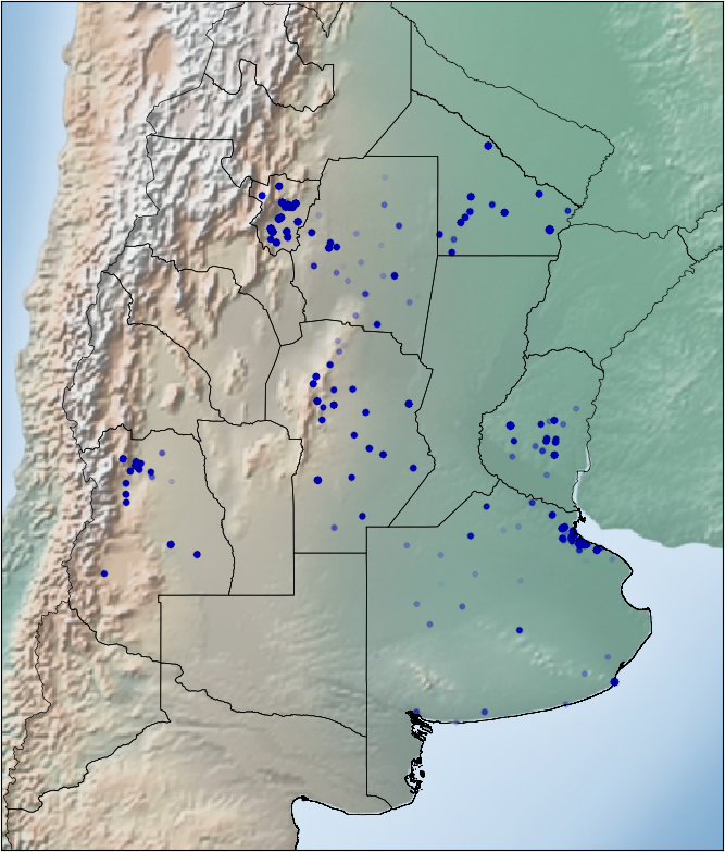
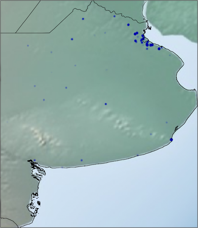
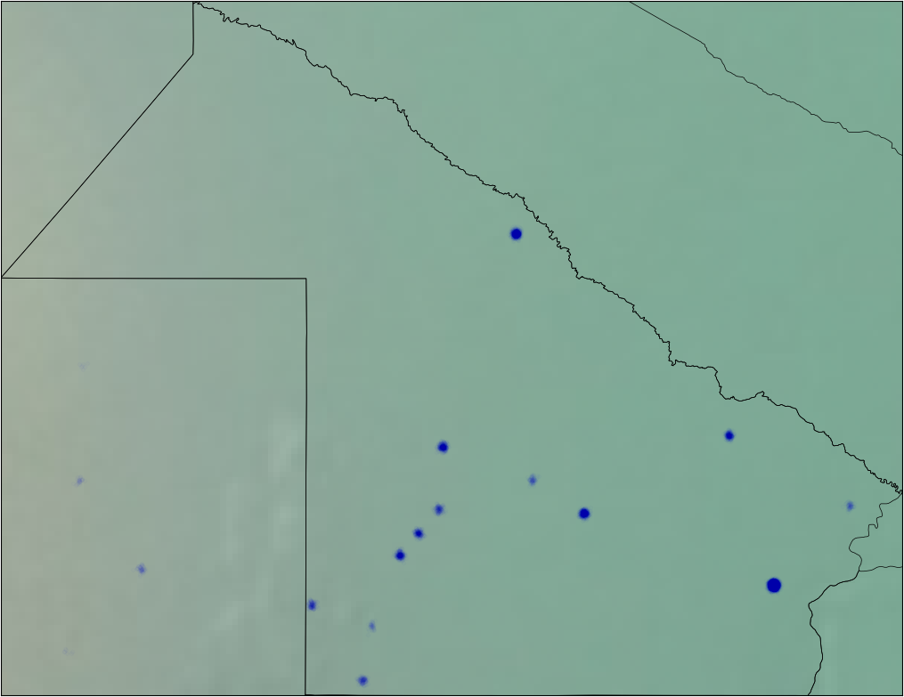
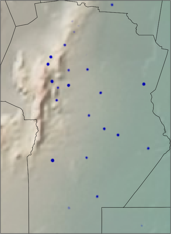
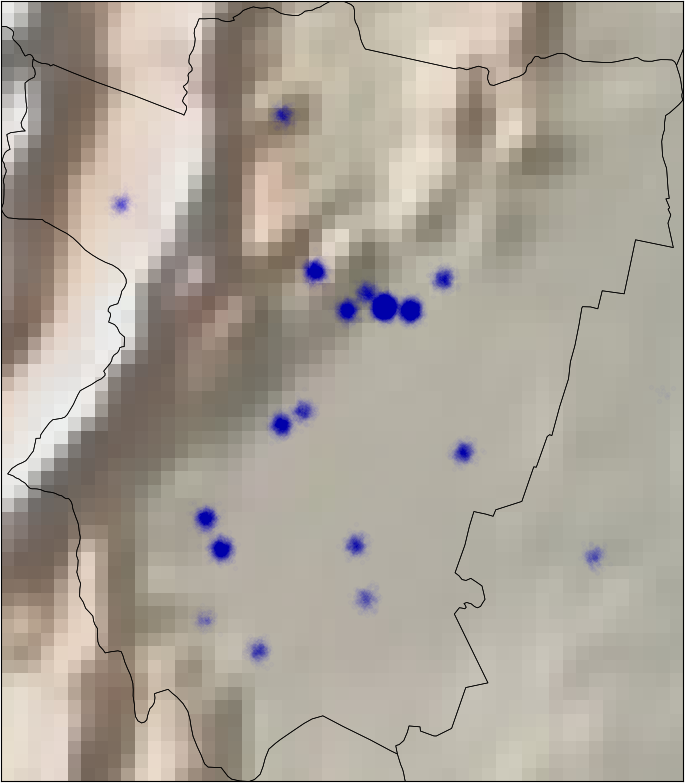
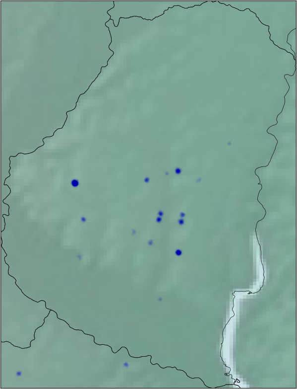
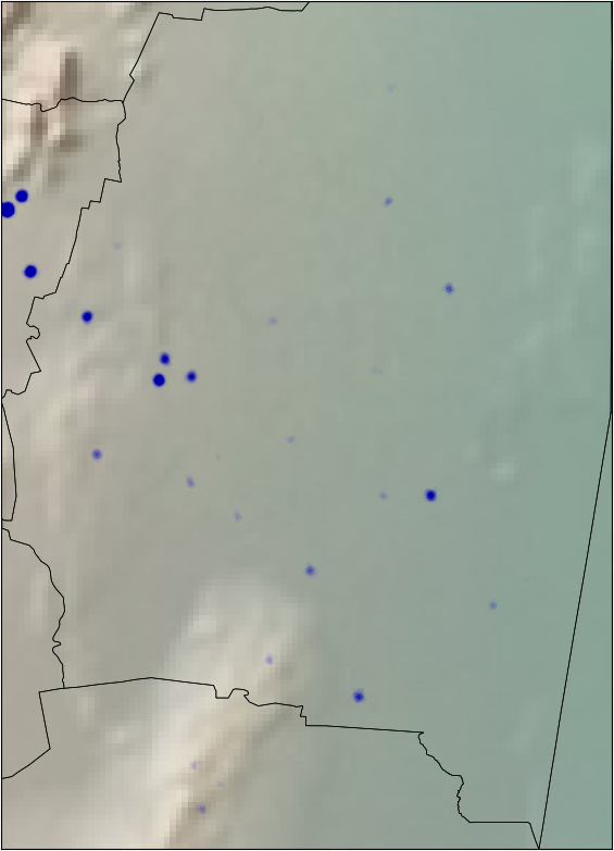
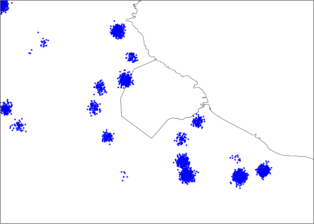
I applied some jitter and alpha blending to the points in the data to be able to see the zones with more or less density of pacients.
Here we have grouped the hospitals only geographically, but we can try one more thing. We can group the hospitals by the ratio of healthy/unhealthy kids using the target variable. For each hospital we count the number of patients that have the target variable in true versus the ones that are false, we divide those numbers and we have a ratio. If the hospital #123 has 80 patients with the target on False and 20 with the target on True, our new feature is r = 0.8. We will see in the next post that this approach was better than the geographic one.
One last and very important thing, we can see that the train data is made of one check-up per row and several patients are repeated. In fact, most of the patients have three or four rows in the train set. Not only that, those patients who have three rows correspond to the same patients that are on the test set. We have the history of the patients in the test set!
In the next post, I’ll continue with these ideas and explain the new features I generated and the predictive models I used to play in the competition.
Thanks for reading!